Physics-based simulation of a pendulum attached to a moveable support point or "anchor block". The support point is assumed to be so massive that it is not affected by the pendulum.
You can drag the anchor block or pendulum with your mouse. Change parameters like gravity, pendulum length, damping, etc. The amplitude and frequency parameters apply a periodic up/down vibrating force.
Try dragging the anchor point by clicking near it with your mouse. Whip it around quickly back and forth -- does the pendulum behave like you would expect?
The math behind the simulation is shown below. Also available: source code, documentation and how to customize.
There are two separate but related simulations happening here:
Kinematics means the relations of the parts of the device, without regard to forces. In kinematics we are only trying to find expressions for the position, velocity, and acceleration in terms of the variables that specify the state of the device.
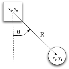
We regard \( y \) as increasing upwards. Begin by using simple trigonometry to write expressions for the pendulum position \( x_1, y_1 \) in terms of the angle \( \theta \) and position of the anchor point \( x_0, y_0 \).
$$x_1 = x_0 + R \sin (\theta) \tag{1}$$
$$y_1 = y_0 - R \cos(\theta) \tag{2}$$
The velocity is the derivative with respect to time of the position.
$$x_1' = x_0' + \theta' R \cos(\theta) \tag{3}$$
$$y_1' = y_0' + \theta' R \sin(\theta) \tag{4}$$
The acceleration is the second derivative with respect to time.
$$x_1'' = x_0'' - \theta'^2 R \sin(\theta) + \theta'' R \cos(\theta) \tag{5}$$
$$y_1'' = y_0'' + \theta'^2 R \cos(\theta) + \theta'' R \sin(\theta) \tag{6}$$
We treat the pendulum bob as a point particle. Drawing the free body diagram for the pendulum bob lets us write an expression for the net force acting on it. Define these variables:
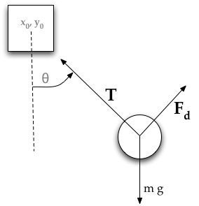
The forces on the pendulum bob are the tension in the rod \( T \), the damping force \( F_d \), and gravity \( -m\;g \). We write separate equations for the horizontal and vertical forces, since they can be treated independently. The net force on the mass is the sum of these.
We can read off from the free body diagram (at left) that the force - acceleration equations (from Newton's \( \mathbf{F} = m \mathbf{a} \)) will be:
$$ m \; x_1''= - T \sin(\theta) + F_d \cos(\theta)$$
$$ m \; y_1''= T \cos(\theta) + F_d \sin(\theta) - m \; g$$
We only need to find the damping force. We assume the damping force is given by the following simple law, which relates the torque to opposite of the angular velocity:
$$\tau = - b \; \theta'$$
One way to imagine the damping force is as a tiny circular spring around the joint where the pendulum attaches to the anchor point; it doesn't matter how long the pendulum is, the same twisting torque is applied. (This is different to how the engine2D system works, where damping is associated with absolute movement through space as well as with rotation.)
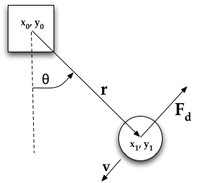
We learn from a physics text book that "The torque acting on the particle with respect to the origin O is defined in terms of the vector (cross) product of r and F as"
$$\tau = \mathbf{r} \times \mathbf{F}$$
One way to look at the above equation: for a given torque, you can use less force at a longer arm length R, or more force for a short arm length R. "Torque is a vector quantity. Its magnitude is given by
$$|\tau| = r F \sin(\gamma)$$
where \( \gamma \) is the angle between \( \mathbf{F} \) and \( \mathbf{F} \). In our case \( \gamma = \pm \pi/2 \), it is always \( \pm 90 \) degrees. We can now write the following expressions for the magnitude of the torque:
$$|\tau| = R F = -b \theta' $$
Solving for the damping force then gives
$$F_d = -\frac{b}{R} \theta'$$
The above is only the magnitude of the damping force. An expression that gives the full directionality of the damping force as a vector is
$$\mathbf{F}_d = -\frac{b}{R} \theta' (\cos(\theta) \mathbf{i} + \sin(\theta) \mathbf{j})$$
Now we can add all the forces: the tension T in the rod, the damping force, and gravity, and express them in 2 dimensional cartesian coordinates, x and y. Here we show the net force and use Newton's law \( \mathbf{F} = m \; \mathbf{a} \).
$$ m \; x_1''= - T \sin(\theta) - \frac{b}{R} \theta' \cos(\theta) \tag{7}$$
$$ m \; y_1''= T \cos(\theta) - \frac{b}{R} \theta' \sin(\theta) - m \; g \tag{8}$$
Now we do some algebraic manipulations with the goal of finding the equation of motion for the pendulum, which will be an expression for \( \theta'' \) in terms of \( \theta, \theta' \). Multiply equation (7) by \( \cos(\theta) \) and equation (8) by \(\sin(\theta)\).
$$ \cos(\theta) m \; x_1''= - T \sin(\theta) \cos(\theta) - \frac{b}{R} \theta' \cos^2(\theta) \tag{9}$$
$$ \sin(\theta) m \; y_1''= T \sin(\theta) \cos(\theta) - \frac{b}{R} \theta' \sin^2(\theta) - m \; g \; \sin(\theta) \tag{10}$$
Add those two equations to get
$$ \cos(\theta) \;m\; x_1'' + \sin(\theta) m \; y_1''= - \frac{b}{R} \theta' - m \; g \; \sin(\theta) \tag{11}$$
Next, substitute equations (5) and (6) for \( x_1'' \) and \( y_1'' \)
$$\begin{multline} \cos(\theta) \;m \Bigl(x_0'' - \theta'^2 R \sin(\theta) + \theta'' R \cos(\theta) \Bigr)\\ + \sin(\theta) m \Bigl(y_0'' + \theta'^2 R \cos(\theta) + \theta'' R \sin(\theta) \Bigr)\\ = - \frac{b}{R} \theta' - m \; g \; \sin(\theta) \end{multline} \tag{12}$$
which simplifies to
$$\cos(\theta) \;m\; x_0'' + \sin(\theta) m \;y_0'' + m\; R\; \theta'' = - \frac{b}{R} \theta' - m\; g\; \sin(\theta) \tag{13}$$
Rearranging this gives the equation of motion for the moveable pendulum
$$\theta'' = -\frac{\cos(\theta)}{R} x_0'' - \frac{\sin(\theta)}{R} y_0'' - \frac{b}{m R^2} \theta' - \frac{g}{R} \sin(\theta) \tag{14}$$
The first two terms are from the motion of the anchor point, \( (x_0, y_0) \). Note that we regard the motion of the anchor point as a "given" here, in line with our assumption that the anchor block is much more massive than the pendulum. The next section considers the separate simulation of the anchor block motion.
The next term, \( -\frac{b}{m R^2} \theta' \) is from the damping force.
The last term \( -(g/R) \sin(\theta) \) is the gravity driving forcing.
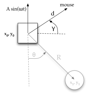
The anchor block has its own separate dynamics from the pendulum. Because we assume that the mass of the anchor block is much greater than the mass of the pendulum, we ignore the effect of the pendulum's motion on the anchor block. We model the anchor block as a point mass that is subject to a strong damping force, to the mouse "rubber band" force, and to an optional vertical oscillating force.
The damping force is \( -b_0 \mathbf{v_0} \) where \( \mathbf{v_0} = (x_0', y_0') \) is the velocity of the anchor block.
The oscillating vertical force is \( A \sin(\omega t) \) where \( t = \) time. The parameters \( A \) and \( \omega \) are available to be set in the controls for the simulation above (the parameters are named amplitude and omega).
The rubber band mouse force is modeled as a spring with zero rest length; it has magnitude of \( k \; d \) and the direction is along the line from the anchor block to the mouse at an angle of \( \gamma \).
Combining these forces with Newton's law \( \mathbf{F} = m \; \mathbf{a} \), we can write the equations of motion for the anchor point:
$$x_0'' = -b_0 x_0' + k d \cos(\gamma) \tag{15}$$
$$y_0'' = -b_0 y_0' + k d \sin(\gamma) + A \sin(\omega t) \tag{16}$$
(We left out any mention of the mass of the anchor block, we can assume that mass is 1).
Note that we can write the following simpler expressions for the mouse force:
$$k d \cos(\gamma) = k (\text{mouse}_x - x_0)$$
$$k d \sin(\gamma) = k (\text{mouse}_y - y_0)$$
Notice that equations (15) and (16) have no influence from the pendulum angle \( \theta \). This means that the anchor point is not affected by the motion of the pendulum at all. This is reasonable since we are told that the anchor point is much more massive than the pendulum.
Between equations (14), (15), and (16) we have our mathematical model of the moveable pendulum.
Essentially we made only one small simple change in the kinematics in equations (1) and (2), which was to add in \( x_0 \) and \( y_0 \). This is the real mathematical difference to the standard pendulum derivation. In that other derivation, we assumed that the anchor point is fixed (and so we could take the short cut of the fixed axis theorem).
Equations (14), (15), and (16) are now close to the form needed for the Runge Kutta method. The final step is convert these three 2nd order equations into six 1st order equations. Define the following first derivatives as independent variables:
Then we can write the six 1st order equations:
$$\begin{multline} \theta' = \Omega \end{multline}$$ $$\begin{multline} \Omega' = -\frac{\cos(\theta)}{R} v_{x_0}' - \frac{\sin(\theta)}{R} v_{y_0}' - \frac{b}{m R^2} \Omega - \frac{g}{R} \sin(\theta) \end{multline}$$ $$\begin{multline} x_0' = v_{x_0} \end{multline}$$ $$\begin{multline} v_{x_0}' = -b_0 v_{x_0} + k (\text{mouse}_x - x_0) \end{multline}$$ $$\begin{multline} y_0' = v_{y_0} \end{multline}$$ $$\begin{multline} v_{y_0}' = -b_0 v_{y_0} + k (\text{mouse}_y - y_0) + A \sin(\omega t) \end{multline}$$Given initial conditions (starting values) for the six variables, we can integrate these differential equations over time to see the evolution of the system.